Holonomy
In the context of a parallel transport defined on a surface it refers to the dependency on the path of a parallel transported vector:
In @needham2021visual page 245 appears this classical example:
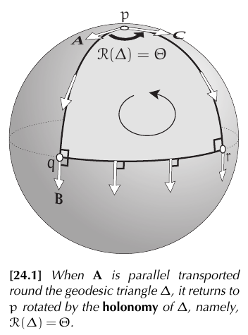
More formally, the holonomy $\mathcal{R}(L)$ of a closed loop $L$ on a surface $S$ is the net rotation of a tangent vector to $S$ that is parallel transported along $L$. Since the angle of two parallel transported vectors remains constant (see parallel transport), we may think of the holonomy as the rotation of the whole tangent plane. It does not depends on where do we begin on $L$.
It turns out that the holonomy around a loop $L$ coincides with the total curvature inside the loop $L$ (for the moment, @needham2021visual page 246). The Gaussian curvature is ultimately equal to the holonomy per unit area.
Local chart
Also, given a chart $\varphi=(u,v)$ for $S$ such that the metric is given in it by
$$ \begin{pmatrix} A^2 & 0\\ 0 & B^2\\ \end{pmatrix} $$then the holonomy of a simple loop $L$ coincides with the circulation of the vector field
$$ V=\frac{\partial_v A}{B} \partial u-\frac{\partial_u B}{A} \partial v $$along $\varphi(L)$:
$$ \mathcal{R}(L)=\mathcal{C}_{\varphi(L)}(\mathbf{V}). $$________________________________________
________________________________________
________________________________________
Author of the notes: Antonio J. Pan-Collantes
INDEX: