On Quantum Mechanics from the beginning

We assume, without definition, the following concepts: there exists a system (in a more general sense than dynamical systems) which is made of states, and we can make measurements of different properties (observables) of the system, obtaining real values which depend on which state the system is. The system changes state (with respect to a parameter $t \in \mathbb N$ or $t\in \mathbb R$ which we call time) according to a dynamical law.

All this can be modelled, at least to my knowledge, in two ways:

Mathematical model 1 (MM1)

• We have a set $\Omega=\{a,b,c,d,\ldots\}$. Its elements are called the pure states of the system. We call this set the phase space.

• The observables are nothing but functions $f: \Omega \to \mathbb{R}$. The measurement process consists, simply, of evaluating the function. It is assumed that the measurement is "clean" in the sense that does not modify the state in which the system is.

• If we have "observables enough" we can have a bijection of $\Omega$ with a "numerical set".

• Probabilities. You can consider that the system is not in a pure state but in a mixed one, a kind of generalized state. As if you have a big box with lots of copies of the system, every of them in a different state. You repeat a measurement several times and you obtain several values, with a distribution of frequencies or probability. To my knowledge, there are two reasons to do this:

1. You are working with too many degrees of freedom (this is the trick of Classical Statistical Mechanics for avoiding too many dimensions.); or

2. You assume that the measurement is not one hundred percent precise, and you repeat again and again obtaining a probability distribution.

• Algebraic formulation: the observables (functions) live inside a complex commutative algebra $\mathcal F$. They can be seen like the main characters of the story, since it is what "we can access". If you can't measure the difference between two systems, you have no right to treat them as different. In mathematics there are lots of examples where a space is recovered from its algebra of functions, or at least from its sheaves. This is the spirit of Algebraic Geometry. Important example: a space is locally compact Hausdorff iff its algebra of continuous functions is a commutative c-star algebra, and reciprocally any commutative c-star algebra is the algebra of continuous functions on some space (the Gelfand spectrum). See @strocchi2008introduction page 15, Gelfand-Naimark theorem. In Classical Mechanics the observables constitute a commutative algebra $\mathcal F$ and the Gelfand spectrum $\Omega$ (multiplicative linear functionals on $\mathcal F$) are the pure states (@strocchi2008introduction page 13). The mixed states are the normalized positive linear functionals. The Riesz-Markov representation theorem let us assure that a mixed state $\omega$ in this sense determines a unique probability distribution $\mu_{\omega}$ on the Gelfand spectrum (see @strocchi2008introduction page 13) such that for an observable $f$

• Dynamics. Once we have the bijection with the numerical set, we usually formulate the dynamical law like a continuous or discrete dynamical system. I have to develop this yet.

Mathematical model 2 (MM2)

• The system consist of a Hilbert space $(\mathcal{H},\langle -,- \rangle)$ whose elements of length 1 (or its rays, I am not sure) are the states of the system.

• The observables are Hermitian operators $\hat Q: \mathcal H \to \mathcal H$. The measurement process, provided we are in state $|\psi \rangle \in \mathcal H$, consists of

• obtaining the basis of eigenvectors $\{|q_i\rangle\}_i$ (with eigenvalues $q_i$) of the operator $\hat Q$.

• randomly selecting one of them, according to the probability distribution $P(|q_i\rangle)=|\langle q_i|\psi\rangle|^2$ , that is, $P(|q_i\rangle)=|c_i|^2$ where $|\psi\rangle=c_1|q_1\rangle+c_2|q_2\rangle+\cdots$

• applying the operator to the selected $|q_i\rangle$ and project the result over $|q_i\rangle$. In general we will call to the operation $\langle \psi |\hat Q |\psi \rangle$ the expected value of $\hat Q$ with respect to $|\psi\rangle$. In the case of eigenvectors this operation returns the eigenvalue.

The measurement has changed the state in which the system is, unless it were in one of the eigenvectors.

• There is something called complete set of commuting observables. If you need more that one observable everything gets complicated, because you have eigenvalues with several eigenvectors (eigenspace of dimension greater than 1) and you maybe have to introduce tensor product to separate then and so on... Think of $x$ coordinate and $y$ coordinate in a discrete setup, for example. Key idea: commuting Hermitian operators have a common basis of eigenvectors. I have to think it more. For the moment, suppose we only need 1 observable.

• Probability is inside the model from the beginning .... it can be added the other sense of probability......... I think

• The observables can be embedded in a c-star algebra $\mathcal A$ which in general is not commutative. I guess that the Gelfand spectrum in this case is the original Hilbert space (pure states). The set of observables corresponds to the subset of $*$-invariant elements of $\mathcal{A}$.

• Dynamical law: since states have length 1, the dynamical

Summary

So to summarize, we can say that:

1. A system (classical system or quantum system) is given by a c-star algebra $\mathcal{A}$. A subset of $\mathcal{A}$ (the $*$-invariants elements) are the observables.

2. Systems can be set on pure states or mixed states. The latter ones are interpreted as a kind of "combination" of the former ones, or better said, probability distributions of them. They are all positive normalized linear functionals on $\mathcal{A}$. The pure states are required to be also multiplicative (also called characters).

3. In the case of a classical system the algebra is commutative. The multiplicative functionals constitute the Gelfand spectrum of $\mathcal{A}$, which is a compact topological space representing the pure states. The rest of the normalized functionals correspond to probability distributions defined on the Gelfand spectrum of $\mathcal{A}$. For pure states, the probability distribution is typically described by a delta function concentrated at a single point in the phase space. This corresponds to the fact that the system is in a definite state, with the position and momentum of each particle in the system being well-defined.

4. In the case of quantum systems, the algebra is not commutative. The multiplicative functionals (pure states) constitute again the Gelfand spectrum of $\mathcal{A}$, which in many important cases, is a complex projective space with an underlying Hilbert space. They can be also interpreted as one-dimensional projections in the algebra, while the general normalized functionals (mixed states) are represented by density matrices, which are positive semi-definite operators with trace equal to 1. I have to think this yet.

Quantum physics as a generalization of classical physics

We can embed MM1 into MM2 in the following way:

• $\Omega$ goes to $\mathbb P \mathbb C^n$, si cardinal de $\Omega$ es $n$

• $f:\Omega \to \mathbb C$ goes to the linear map

defined like the diagonal matrix whose entries are the values of $f$.

• and so on... (I have to write this better)

• ...

But, why do we care about this embedding of MM1 into MM2? Why don't we settle for MM1? See this note: Why did physics go quantum

To review and maybe incorporate: as it is said in this MO answer the point of QM is to see the algebra of functions as "immersed" in a bigger not necessarily commutative algebra.

Old latex notes, to incorporate above one day...

With classical probability

We are going to analyse, from the beginning, the Stern-Gerlach experiment from a mathematical viewpoint, and try to see why is natural the formulation of QM. Imagine that electrons have an internal configuration that can be observed with a Stern-Gerlach device ($SG$) when they are shot with an electron gun. We align the machine with the $z$ axis (we call this configuration $SG_z$) and it gives us two outputs when electrons arrive: for example, red and green. Our first idea would be to think that there are two kinds of electrons or two states of the electron.

From the point of view of set theory, improved with basic probability theory, our first thought is: "ok, I have a set of electrons $\tilde{\Omega}$ and a map that sends their elements to the set $\{r,g\}$ with different frequencies. So, since there are (approximately) an infinite number of electrons, I can take a partition of $\tilde{\Omega}$ and shrink all data to a new set $\Omega=\{r,g\}$ with a probability measure $P$, and we would have no loss of information.

Then, we observe that if we have a copy of this machine and rotate it (or keep it fixed and rotate the gun that shoot the electrons in the opposite direction) to the $x$ axis (let's call $SG_x$ to this second machine) then we obtain two other outputs (big and small, for example) with a new probability distribution $P'$. If we assume a classical behavior of the states of the electron, i.e., we can use machine $SG_z$ on an electron and then machine $SG_x$ on the same electron and that does not change the state itself, we can obtain a joint probability distribution $\tilde{P}$, and conclude that there are four different states:

with a new probability function. Our new set appears like a cartesian product of the previous "sets of possibilities".

Observe that the joint distribution is not necessarily

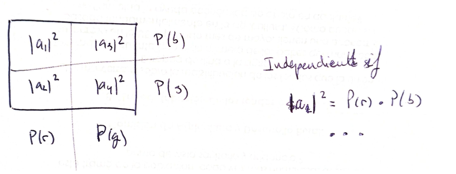
being this the case only when the variables are independent. For example, maybe there is a correlation between being red and being big.

A different approach

All of this could have been translated to maths in a very different way, far more complicated, but that it will pay off later.

A finite set $B$ with $N$ elements can be viewed as a Hilbert space

with inner product

This way we have "enriched" the set:

1. we conserve the original elements of the set, codified in the rays through the canonical basis; but we get new objects, the superposition of the elements. This new objects may not have an interpretation for us, at a first glance.

2. And we also have a measure of "how independent" this objects are: the inner product. For example, the original elements are totally independent, for their inner product is 0.

Let's come back to Stern-Gerlach. Instead of thinking as before in the set $\Omega=\{r,g\}$, we take the Hilbert space

with the usual inner product.

The canonical basis elements of $\mathcal{H}_1$ (or better said, the rays through them) will represent the states $r$ and $g$, and the probability function $P$ will be encoded in a unitary vector $s_1 \in \mathcal{H}_1$ (or better said, the ray through it) in such a way that

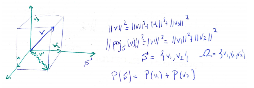
represents the probability of obtaining the output $r$ when using the first machine. And the same for $g$. Observe that we are treating on an equal footing the states ($r$ or $g$) and the probability measure.

So far, two questions can arise:

• We have chosen in $\mathcal{H}_1$ the usual inner product (equivalent to $\|\cdot \|_2$). Why not other inner product or even why not a more simple set up like an absolute value norm? That is, why don't we take, for example, $\|v\|_1=|v_1|+|v_2|$ and encode probabilities in $\|proj_r(s_1)\|_1$ without the square? Well, the only $p$-norm satisfying the parallelogram rule is $\|\cdot\|_2$, and this rule is needed to form an inner product from the norm. The finer approach of inner product will be needed later because it let us use further mathematics concepts (orthogonality, unitary Lie groups,...). Moreover, even intuitively the inner product approach is desirable because it gives us a measurement of the independence of the elements represented by the rays in the Hilbert space.

• Why don't we use real numbers and take as probabilities the absolute values of the component instead of the square? Once we fix the use of the 2-norm, we need to deal with amplitudes (i.e., numbers whose square give probabilities) because we want to keep with us the addition of probabilities for incompatible events, from the classical setup.

• And also, why complex numbers in QM?

Within this approach to sets as Hilbert spaces, subsets are encoded as subspaces, the union of sets is translated as the direct sum of subspaces, intersection of sets as intersections of subspaces and the complement of a set as the orthogonal complement of the subspace.

Random variables vs operators

Let's continue with $(\mathcal{H}_1, \langle | \rangle{}{})$. If we had numerical data instead of qualitative one (i.e., suppose that instead of "red" and "green", our machine give us two fixed values 0'7 and 1'8, or in other words, a random variable) we would codify this, within this new approach, in the idea of an operator. That is, a linear map

such that

i.e.,

The random variable registers the idea of a measurement. This new approach to them may look very artificial, but it retains the same information that the classical probability approach:

• We recuperate the values, for example for $r$, with

• The expected value of $F$, provided that probabilities are given by the vector $s_1$, would be

When we take our second machine $SG_x$ we have other Hilbert space, say $\mathcal{H}_2$, and other state $s_2 \in \mathcal{H}_2$ encoding probabilities of $b$ and $s$. Suppose that this machine also gives numerical values, so that we have another operator $G:\mathcal{H}_2\mapsto \mathcal{H}_2$, also diagonal in the canonical basis of $\mathcal{H}_2$.

If we assume, as before, a classical behavior of the states, we can model this with a new Hilbert space

whose basis will be denoted by $\{rb, rs, gb, gs\}$. This tensor product plays the role of cartesian product in the previous set up.

We can think that the state describing the system would be

but in fact this is only an special case when the two machines are yielding the equivalent to "independent variables" (the joint probability is the product of the probabilities). In general, it is valid any $\Psi \in \mathcal{H}_1 \otimes \mathcal{H}_2$ provided that the coefficients in the linear combination

are such that

where the second and the fourth equations could be deduced, so we can remove it.

The random variable represented by the operator $F$ corresponds here to $F\otimes Id$ (Kronecker product), and $G$ to $Id \otimes G$.

Quantum behavior

We are yet in a classical set up, but now we are going to jump to the quantum behavior. Nevertheless, what have been said so far would be valid, even in QM, for observables that are "totally independent" (own terminology), for example, $x$ position and $y$ position. I think the technical name is commuting observables.

Suppose that after measuring an electron with the first device we obtain $r$. Then we use the second one and obtain $b$. In a classical setup we would expect that if we use device 1 again, we obtain $r$ again, but this is not what happens with Stern-Gerlach devices. We obtain $r$ and $g$ with certain frequencies (although fixed).

The logical explanation (at least from the point of view of QM) is to accept that electron is in a certain state $\Psi \in \mathcal{H}_1$ before the use of any machine. Until now, we have assumed that the vector in the Hilbert space encodes probabilities. But now we are saying that the electron is the vector (or, at least, a part of the electron). Every time we use a machine, the vector $\Psi$ moves to a new location. For example: we use machine 1 and get $r$ or $0'7$ (with certain probability), so the state vector has travelled to $r$. If we use machine 1 again we obtain the same result: probability of obtain $r$ again is the length of the projection of $r$ on $r$, that is, 1!! If we use machine 2, depending on the value obtained, the state vector travels to $b$ or $s$ but they are still inside $\mathcal{H}_1$.

That is, we have machines (or one machine with different positions) that extract information of the system. The system is codified in a Hilbert space and the machines in operators. Every operator has privileged states with good behavior respect to it (a "classic behavior" respect to it, we can say). That is the reason why we cannot consider any operator, but the corresponding to Hermitian matrices.

If the system is in a "classical state" for the operator, the operator will only change the scale of the state vector, and the measurement arises when we check the length of the transformed vector

If the system is in a "non-classical" state for this machine, it goes to the "most similar" classical state for the machine (not for sure, but with a probability that depends on the similitude), and then the above is applied.

Can we find the expression of the privileged states of a machine with respect of the ones of the other? That is, who are $b$ and $s$ (canonical base for machine 2) in the canonical base of $\mathcal{H}_1$?

Suppose the machines are $SG_z$ and $SG_x$ in the Stern-Gerlach experiments. According to the measured probabilities in Stern-Gerlach experiment we could assign the coefficients:

The choice of the coefficients is arbitrary but subject to the measured probabilities.

Observe that, so far, we have no need of complex numbers.

Of course, the operator $SG_z$ has the matrix expression in "its associated basis" is (we are assuming now that the outputs are 1 and -1 instead of 0'7 and 1'8):

What is the matrix expression for the $SG_x$ machine in this basis? Since $SG_x b=b$ and $SG_x s=-s$, solving a very easy linear system we find that

But we can think like if we have an infinite number of machines $SG_{\theta}$. They are all the same that our original $SG_z$ but rotated an angle $\theta$ from the $z$ axis towards the $x$ axis. For the moment, we will be pretending that the universe is of dimension 2. With each of these machines we get two results, say $M$ and $B$, and empirically obtain that, once our system is in state $M$, $SG_z$ yields an expected value of $cos(\theta)$, what is reasonable even from the classical point of view. If we write $M=\alpha r +\beta g$ and $B=\gamma r+ \delta g$, since

(expected value) and $M$ is normalized, i.e.,

we obtain

In a similar way, since the expected value for $B$ is $-cos(\theta)$ and $M$ and $B$ must be orthogonal we can conclude

Solving a linear system we find the matrix for $SG_{\theta}$:

So, in conclusion, we can assume that when we rotate the $SG_z$ machine an angle $\theta$ the well-behaved states are now

that is, the privileged vectors are rotated an angle of $\theta/2$. Or we can interpret that if we rotate the system (our electron gun in state $r=\begin{pmatrix}1 \\0 \end{pmatrix}$) an angle of $-\theta$, we are putting the electron in a state

And the operator goes from

to

This let us predict probabilities in the Stern-Gerlach experiment: what would be the probability of obtain such result if we turn the machine such angle? It is a numerical model for this family of Stern-Gerlach experiments.

But we can think in it like a geometric model, too. The different directions of space (plane, in this case) are codified in the matrices $SG_{\theta}$: $SG_z$ would represent the unit vector along $z$ axis, and $SG_{\theta}$ is the result of a rotation of angle $\theta$. And we are led to think that spin is an "internal object" inside the electron with a special kind of symmetry without counterpart in classical-macroscopic terms.

(see section \textit{About spin})

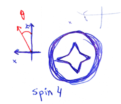
So, what about our electron? After performing a rotation of angle $\theta$ the privileged states of the Hilbert space have rotated $\theta/2$ so we come back to the initial configuration after a $4\pi$ rotation. So we can say that electron has spin 1/2. It is a bit difficult to visualize but you can imagine an arrow with a flag attached in such a way that the flag turns half the angle of the arrow.

On the other hand, observe that the matrices

behaves like a orthogonal vector basis of $\mathbb{R}^2$. In fact

among other similarities. But the matrices product gives them an additional intrinsic algebra structure which the vector space $\mathbb{R}^2$ lacks. What does it mean, geometrically?

There is a correspondence between the subalgebra generated by the matrices $\{SG_z, SG_x\}$ and the abstract Clifford algebra of dimension 2 and positive signature with orthonormal basis $\{e_1, e_2\}$. Since we know that in the Clifford algebra the even subalgebra acts over $\mathbb{R}^2$ like rotations (on the "sandwich way") we are led to think that internal states of the electron are elements of $\mathcal{G}_2^+$, that is, spinors. That is, the element

is identified with the pair of elements of the Hilbert space

One observation: the even subalgebra behaves like complex numbers. So the complex numbers have already entered the scene.

The 3-dimensional space

But the Universe is not planar, is 3D. What happens when we rotate the machine out of the $xz$-plane? Experiments show that the pure $y$ orientation of the machine ($SG_y$) yields a pair of states, call it head and tail, $h$ and $t$, with probabilities similar to those of the $SG_x$ ($b$ and $s$) when throwed through $SG_z$. But keep an eye: further experiments show that those are not the privileged states of $SG_x$. This cannot be, definitively, modelled if we stay with real numbers (see page Why complex numbers in QM).

We can solve this problem by using complex coefficients, and in this way we arrive to the picture of the internal states as elements of $SU(2)$. Indeed, the measured probabilities together with the restrictions of orthonormality of $h$ and $t$ lead us to

If we now measure probabilities respect to $SG_x$ (i.e., probabilities of $b$ and $s$ output when we feed the machine with $h$ or $t$ states) we can find that $\alpha=\pi/2$. That is,

And with some computations we get

The matrices $SG_x, SG_y, SG_z$ are called Pauli matrices.

In conclusion, we have a machine, $SG$, that can be oriented in any spatial direction, $\hat{n}$ (unitary vector). When we fix this direction we get a matrix, $SG_{\hat{n}}$, that encodes all the data of the machine (final states, obtained values and probabilities) with this direction. This matrix has two eigenvectors of $\mathbb{C}^2$, $\ket{n+}$ and $\ket{n-}$, that represent the state of the electron after passing through the machine. Or we can think that the device $SG$ is fixed, and we turn the electron gun to a new spatial orientation $\hat{n}$. Internally for the electron this has an effect: if it was at state

it is arriving to a new state

that can be computed like this:

• The rotation of the gun is performed with a $3\times 3$ orthogonal matrix $R\in SO(3)$, that can be viewed as an element of $SU(2)$ (in fact, there are two of them, since it is a double covering).

• In this assignation we can observe a kind of "miracle". The matrix $R$ can be obtained like the product of other three

where $\{G_x, G_y, G_z\}$ are $3\times 3$ matrices forming a basis of $so(3)$. To find the corresponding element of $SU(2)$ we use the isomorphism (as Lie algebras) of $so(3)$ with $su(2)$, and then the exponential map over $SU(2)$. And the miracle is that the images of $G_x,G_y,G_z$ are

although this matrices (without the $i$) appeared like operators to encode data of an observable, not like transformations!!!

• The obtained element of $SU(2)$ rotates the initial "internal vector" $\begin{pmatrix}1\\0\end{pmatrix}$ in the usual way: complex matrix product.

• If we had chosen the other element of $SU(2)$ we would have arrived to other vector in $\mathcal{H}$. But the states are not elements of $\mathcal{H}$, but of $\mathbb{P}(\mathcal{H})$.

Some considerations to further thoughts:

• The element of $SU(2)$ applied in the sandwhich way to the matrices $SG_n$ rotates them, i.e., gives the same result that applying an usual 2x2 rotation matrix on the left. This aims to think the matrices $SG_n$ like vectors...

• In the point 2 above we watch that $i SG_n$ behaves like bivectors in a Clifford algebra, so here is other reason to think that $SG_n$ are vectors.

• All would be, therefore, simpler if we forget the Pauli matrices and go to Clifford algebras¿?

• Explicit computations can be found at mathematica file \textbf{quantum computations SPIN12}

________________________________________

________________________________________

________________________________________

Author of the notes: Antonio J. Pan-Collantes

antonio.pan@uca.es